Scalable in-database Machine Learning & NLP with PL/Python

This blog constitutes the third part of the Greenplum for End-to-End Data Science & ML series. In this article, we demonstrate combining Greenplum Data Warehouse MPP capabilities with Python’s rich ecosystem to make the end-to-end Machine Learning / NLP model development experience significantly faster.
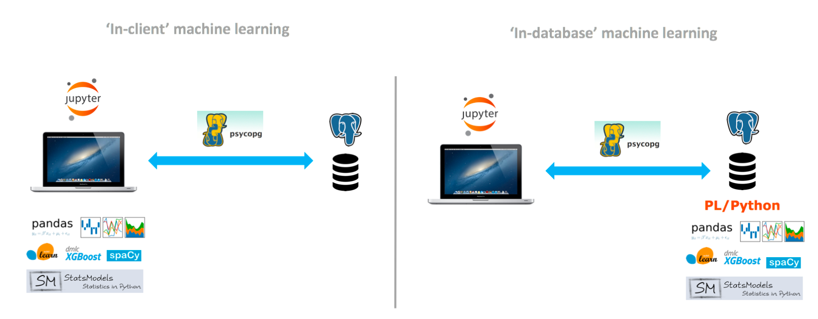
The figure below illustrates a much-needed paradigm shift when training and inferencing ML models on real-life, large datasets.
- In-client machine learning requires data movement from the data source to the computing environment, but this approach becomes prohibitive when the amount of data used is large (e.g. 10s of GBs ~ PBs).
- In-database machine learning pushes the computing down to the data source, eliminating data movement and significantly increasing scalability and performance.
Setup and connectivity
1. Install Packages
pip install ipython-sql pandas numpy sqlalchemy plotly-express sql_magic pgspecial
2. Import Packages
    import pandas as pd
    import numpy as np
    import os
    import sys
    import plotly_express as px
    # For DB Connection
    from sqlalchemy import create_engine
    import psycopg2
    import pandas.io.sql as psql
    import sql_magic
3. Database Connectivity
There are several ways to establish a connection to Greenplum. With a Jupyter notebook, one can use SQL magic. This allows running SQL queries in a Jupyter cell. Link to documentation: https://pypi.org/project/ipython-sql/ Installation on the client:
pip install ipython-sql
For use at the notebook level, it suffices to establish the connection:
    %load_ext _ sql
    %sql postgresql://<user>:<password>@<IP_address>:<port>/<database_name>
Then run the SQL commands in a cell like this:
    %%sql
    SELECT version ();

You can also use the psycopg2 connector or pyodbc (there are also other options via JDBC, for instance)
Dataset Overview
The dataset consists of 1967 stock market financial news written in English and categorised by sentiment.
Data Fields are:
- docid: the unique identifier of financial news
- original_news: raw text of financial news
- label: a label corresponding to the class as a string: positive or negative
    %%sql
    SELECT * FROM ds_demo.sentiment_news
    LIMIT 5;

%sql SELECT count(*) FROM ds_demo.sentiment_news;

NLP — Sentiment Analysis with PL/Python
Sentiment analysis aims to determine the sentiment strength from a textual source for sound decision-making; it’s widely used in financial companies to predict whether the news may positively or negatively influence the future stock price.
First, we’ll explore and visualise our dataset, combining SQL with Pandas & Plotly Python packages.
1. Sentiment classes distribution of our dataset:
%%read_sql df_count_sentiment
SELECT label, count(*) AS number_of_news
FROM ds_demo.sentiment_news
GROUP BY 1
ORDER BY 2 ASC

color_discrete_map = {'negative': 'rgb(255,0,0)',
'positive': 'rgb(0,255,0)' }
px.pie(df_count_sentiment,
values = 'number_of_news',
names = 'label',
color = 'label',
color_discrete_map=color_discrete_map)
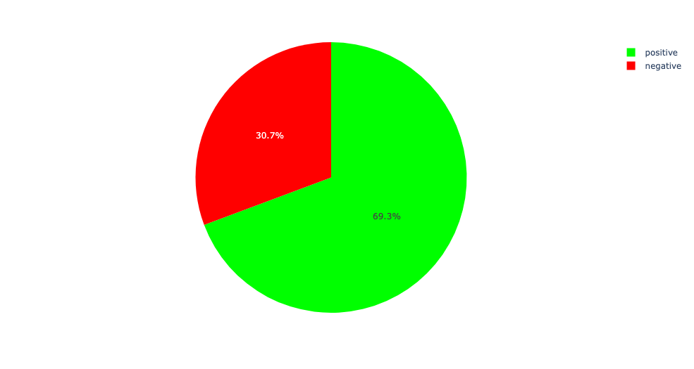
The chart shows that our dataset is imbalanced; we have twice as positive news than negative news. This can impact our model performance and might result in underfitting in real-life data science projects.
2. Number of Characters
    %%read_sql df_max_length
    SELECT max(length(original_news))
    FROM ds_demo.sentiment_news;

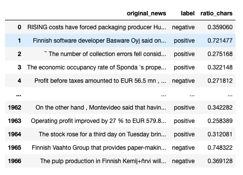
The most extended news of our dataset has less than 300 characters, which means that the sentiment can be captured from a short and synthetic text.
3. Number of characters by sentiment class:
    %%read_sql df_len_news
    SELECT original_news,
           label,
           length(original_news) * 1.0 / max(length(original_news))
           OVER (partition by NULL) AS ratio_chars
    FROM ds_demo.sentiment_news
    px.box(df_len_news,
           y="ratio_chars",
           x ='label',
           color='label',
           title = 'Number of characters distribution by sentiment class',
           color_discrete_map=color_discrete_map)
4. Number of words by sentiment class:
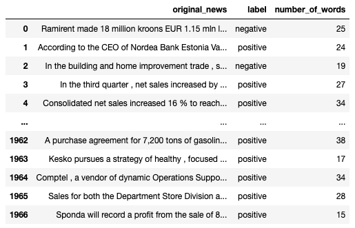
    %%read_sql df_len_words
    SELECT original_news, label,
           ARRAY_LENGTH(STRING_TO_ARRAY(original_news, ' '), 1)
           AS number_of_words
    FROM ds_demo.sentiment_news
        y="number_of_words",
        x ='label',
        color='label',
        title = 'Number of words distribution by sentiment class',
        color_discrete_map=color_discrete_map)
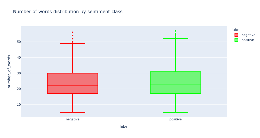
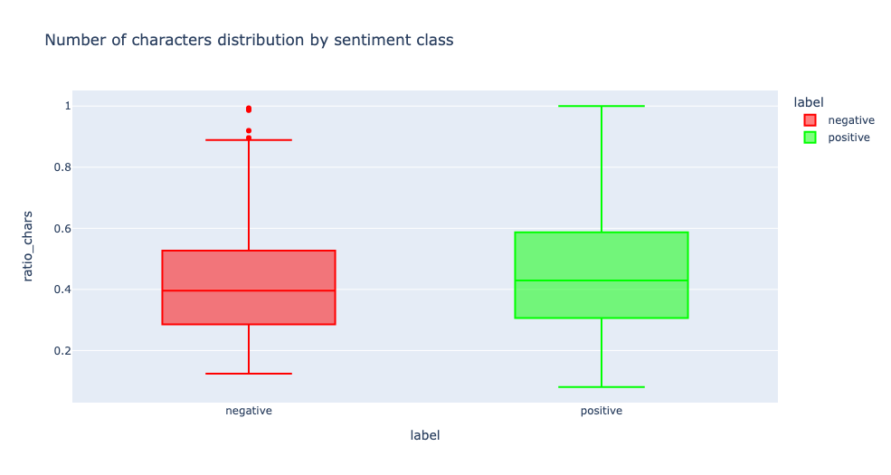
Positive news tends to have slightly more words and characters than negative news, but overall we can’t base our analysis on length.
Data Preprocessing — Text Cleaning
Text cleaning here refers to removing or transforming specific parts of the text so that the text becomes more easily understandable for NLP models learning the text. This often enables NLP models to perform better by reducing noise in text data.
To do that, we create a PL/Python and apply simple preprocessing actions:
- Firstly, change texts to lowercase.
- Then, delete any special characters and URLs.
- Finally, delete any multiple spaces.
    %%sql
    DROP FUNCTION IF EXISTS text_prepare(text);
    CREATE OR REPLACE FUNCTION text_prepare( content text)
    RETURNS text
    AS $$
        import re
        text = content
        replace_by_space_re = re.compile('[/(){}\[\]\|@,;]')
        bad_symbols_re = re.compile('[^0-9a-z #+_]')
        links_re = re.compile('(www|http)\S+')

        text = text.lower()  # lowercase text
        text = re.sub(replace_by_space_re," ",text)
        text = re.sub(bad_symbols_re, "",text)
        text = re.sub(links_re, "",text)
        text = re.sub(' +', ' ', text)
        return text.strip()
    $$ LANGUAGE plpython3u
    ;
We store processed news in a new column called cleaned_text, which will be used for model training.
    %%sql
    ALTER TABLE ds_demo.sentiment_news ADD COLUMN cleaned_text text;
    UPDATE ds_demo.sentiment_news
     SET cleaned_text = text_prepare(original_news::text);
A quick overview of cleansed news:
%sql SELECT * FROM ds_demo.sentiment_news LIMIT 2;

Train a Sentiment Analysis model with PL/Python
Training a Natural Language Processing model to automatically predict the Sentiment of financial news can help traders and investors to build their trading/quantitative strategies.
Sentiment analysis is a text classification task. In this section, we use the Bag of Words technique to convert texts into numerical representation such that the same can be used to train a Logistic Regression model.
Model training — Term Frequency Logistic Regression
Let’s write PL/Python function that can be called like any other SQL function. The integration is effortless, as Python has endless libraries for Machine Learning.
Moreover, besides giving full support to Python, PL/Python also provides convenient functions to run any parametrised query. So, executing Machine Learning algorithms can be a question of a couple of lines.
Let’s take a look:
    %%sql
    DROP FUNCTION IF EXISTS train_sentiment_news(text[],text[]);
    DROP TYPE IF EXISTS news_type;
    -- Create a new type for our PL/Python function output
    CREATE type news_type AS (content text, label text, prediction text);
    -- PL/Python function using Python3.9
    CREATE FUNCTION train_sentiment_news( cleaned_text text[], label text[])
    RETURNS SETOF news_type
    AS $$
        import pandas as pd
        from sklearn.feature_extraction.text import CountVectorizer
        from sklearn.model_selection import train_test_split
        from sklearn.linear_model import LogisticRegression

        X = cleaned_text
        y = label
        df= pd.DataFrame()
        df['content'] = X
        df['label'] = y
        X_train, X_test, y_train, y_test = train_test_split(df['content'], df['label'], test_size=0.2, random_state=42)

        vectorizer = CountVectorizer(min_df=4, stop_words='english')

        X_train = vectorizer.fit_transform(X_train)
        X_test = vectorizer.transform(X_test)

        # LOGISTIC REGRESSION
        logreg = LogisticRegression()
        # TRAIN
        logreg.fit(X_train, y_train)
        X = vectorizer.transform(df['content'])
        # PREDICTIONS ON FULL DATASET
        lr_prediction = logreg.predict(X)
        df['prediction'] = lr_prediction

        return [{'content': str(row['content']),
                 'label': str(row['label']),
                 'prediction': str(row['prediction'])}
                for index, row in df.iterrows()]

    $$ LANGUAGE plpython3u;
As you can see, PL/Python is straightforward.
- Firstly, we import the packages we need; we use pandas and scikit-learn libraries.
- We need to load inputs (news and labels) into a dataframe and transform the numeric variables into numeric type using Bag of Words / CountVectorizer
- Then, we call Logistic Regression and train it on the training set (80% of our dataset).
- Finally, we return the prediction on the whole dataset as a list of news_type types.
The final line specifies the extension language: in this case, we are using Python3, and for that reason, the extension is called plpython3u. If you want to execute it in Python2, use the extension language named plpythonu.
Greenplum also provides another language handler, PL/Container, which runs PL/Container in a Docker. The execution could indeed be safer.
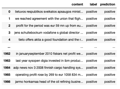
Show predictions
We can check predictions made by our model.
The function train_sentiment_news() takes two arrays as inputs, so we need to apply ARRAY_AGG() function to concatenate all records of columns cleaned_text and labels together as two arrays.
Furthermore, since train_sentiment_news() returns a set of new_type, we need to decompose every record of results into different columns using CTEs (Common Table Expression).
    %%read_sql df_preds
    WITH cte_data_array_agg AS (
            SELECT ARRAY_AGG(cleaned_text) AS contents,
                    ARRAY_AGG(label) AS labels
            FROM ds_demo.sentiment_news
        ),
        cte_predictions AS (
            SELECT train_sentiment_news(t.contents, t.labels)
            FROM cte_data_array_agg
        )
    SELECT (train_sentiment_news::news_type).* FROM cte_predictions;
Model Evaluation
Now, let’s evaluate our model by calculating: Accuracy, F1-score, Precision, Recall
    %%sql
    DROP FUNCTION IF EXISTS metrics_report(text[],text[]);
    DROP TYPE IF EXISTS prediction_type;
    CREATE type prediction_type AS (accuracy float, f1_score float, precision float, recall float);
    CREATE OR REPLACE FUNCTION metrics_report(label text[], prediction text[])
    RETURNS prediction_type
    AS $$
        from sklearn.metrics import precision_recall_fscore_support as score
        from sklearn.metrics import accuracy_score
        import numpy as np

        y_true = label
        y_pred = prediction

        accuracy = accuracy_score(y_true, y_pred)
        precision, recall, f1_score, support = score(y_true, y_pred)

        precision = float(np.mean(precision))
        f1_score = float(np.mean(f1_score))
        recall = float(np.mean(recall))
        accuracy = float(accuracy)

        return {'accuracy': accuracy,
                'f1_score': f1_score,
                'precision': precision,
                'recall': recall
        }
    $$ LANGUAGE plpython3u
    ;
We apply ARRAY_AGG() to concatenate columns and decompose composite-type results using CTEs.
    %%read_sql df_preds
    WITH
      cte_data_array_agg AS (
        SELECT ARRAY_AGG(cleaned_text) AS contents, ARRAY_AGG(label) AS labels
          FROM ds_demo.sentiment_news
      ),
      cte_predictions AS (
          SELECT train_sentiment_news(t.contents, t.labels)
          FROM cte_data_array_agg
      ),
      cte_label_pred AS (
        select (train_sentiment_news::news_type).*
          FROM cte_predictions
      ),
      cte_metrics_report AS (
          SELECT metrics_report(array_agg(label), array_agg(prediction))
          FROM cte_label_pred
      )

    SELECT (metrics_report::prediction_type).* FROM cte_metrics_report

The model has achieved an accuracy of 92.93%, whereas recall and precision are slightly lower than accuracy.
Model Deployment — Storing the model
It doesn’t make much sense to create a model and not do anything with it. So, we will need to store it as binaries using the “bytea” data type.
Store it as binary in a SQL table
    %%sql
    DROP FUNCTION IF EXISTS save_nlp_models(text[],text[]);
    DROP TYPE IF EXISTS model_type CASCADE;
    CREATE TYPE model_type as (model_logreg bytea, model_bow bytea);
    CREATE FUNCTION save_nlp_models(cleaned_text text[], label text[])
    RETURNS model_type
    AS $$

        import pandas as pd
        from sklearn.feature_extraction.text import CountVectorizer
        from sklearn.model_selection import train_test_split
        from sklearn.linear_model import LogisticRegression
        import pickle

        X = cleaned_text
        y = label
        df= pd.DataFrame()
        df['content'] = X
        df['label'] = y
        X_train, X_test, y_train, y_test = train_test_split(df['content'],
                                                            df['label'],
                                                            test_size=0.2,
                                                            random_state=42)

        vectorizer = CountVectorizer(min_df=4, stop_words='english')

        X_train = vectorizer.fit_transform(X_train)
        X_test = vectorizer.transform(X_test)

        # LOGISTIC REGRESSION
        logreg = LogisticRegression()
        logreg.fit(X_train, y_train)
        X = vectorizer.transform(df['content'])
        lr_prediction = logreg.predict(X)
        df['prediction'] = lr_prediction

        # Save Logistic Regression model
        model_logreg = pickle.dumps(logreg)
        # Save CountVectorizer
        model_countvectorizer = pickle.dumps(vectorizer)

        return {'model_logreg': model_logreg
                ,'model_bow': model_countvectorizer}
    $$ LANGUAGE plpython3u
    ;
To do so, let’s create a table ds_demo.saved_models to save the model first:
    %%sql
    DROP TABLE IF EXISTS ds_demo.saved_models;
    CREATE TABLE ds_demo.saved_models (model_logreg bytea,
                                       model_bow bytea,
                                       model_name text);
In this case, our table has just a model_name and two byte array fields (one for Logistic Regression and the other for Bag of Words) that is the actual model serialised. Please note that it is the same data type as the one that our defined Scikit-learn models return.
Once we have the table, we can easily insert a new record with the model:
    %%sql
    WITH cte_models AS (
            SELECT save_nlp_models(t.contents, t.labels)
        FROM (
            SELECT ARRAY_AGG(cleaned_text) AS contents,
                   ARRAY_AGG(label) AS labels
              FROM ds_demo.sentiment_news) t
          ),
        cte_casted_model AS (
            SELECT (save_nlp_models::model_type).*
            FROM cte_models)

    INSERT INTO ds_demo.saved_models
    SELECT model_logreg, model_bow, 'nlp_sentiment_analysis_bow_logreg' AS model_name FROM cte_casted_model;
Show binaries
    %%sql
    SELECT model_name, model_logreg::text, model_bow::text
    FROM ds_demo.saved_models;

Displaying Model Info
So far, we have been able to create a model and store it. But getting it directly from the database isn’t very useful.
Therefore, we must return to Python to display useful information about our model. This is the function we are going to use:
    %%sql
    DROP FUNCTION get_model_info(text,text,text);
    CREATE OR replace FUNCTION get_model_info(model_table text, model_column text, model_name text)
    RETURNS text
    AS $$
        from pandas import DataFrame
        import pickle
        rv = plpy.execute('SELECT %s FROM %s WHERE model_name = %s;' % (plpy.quote_ident(model_column), model_table, "'"+model_name+"'"))
        model = pickle.loads(rv[0][model_column])

        return str(model.get_params())

    $$ LANGUAGE plpython3u;
Let’s start from the beginning: we are passing, again, the table containing the models and the column that holds the binary. The pickle.load() function reads the output.
(Here, you can see how results from a plpython query plpy.execute are loaded into Python).
Once the model is loaded, we return model.get_params(), where our logistic regression parameters are stored.
This is just an example of how to output a specific model feature. You can create similar functions to return other features or even all features.
Let’s take a look at what it returns:
    %%sql
    select get_model_info('ds_demo.saved_models','model_logreg','nlp_sentiment_analysis_bow_logreg');

Model inference — predict new data-feed
Now that we have a model let’s use it to make predictions! Invoking the model is simple and can be done in SQL using PL/Python.
    %%sql
    DROP FUNCTION IF EXISTS predict_sentiment(text, bytea, bytea);
    CREATE FUNCTION predict_sentiment(cleaned_text text, model_logreg bytea, model_bow bytea)
    RETURNS text
    AS $$
        import pickle

        logreg = model_logreg
        vectorizer = model_bow
        texts = cleaned_text

        # Save Logistic Regression model
        model_logreg_bytes = pickle.loads(logreg)
        # Save CountVectorizer
        model_countvectorizer = pickle.loads(vectorizer)

        return list(model_logreg_bytes.predict(model_countvectorizer.transform([texts])))[0]
    $$ LANGUAGE plpython3u
    ;
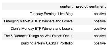
Compared to the previous function, we add one input parameter (cleaned_text), passing the input representing a piece of financial news for which we want to get the sentiment.
    %%sql
    SELECT content, predict_sentiment(text_prepare(t.content), b.model_logreg, b.model_bow)
    FROM
       ds_demo.financial_news t,
        ds_demo.saved_models b
    LIMIT 5;
We can now process larger datasets and show positive/negative news distribution.
    %%sql
    SELECT predict_sentiment, count(*)
    FROM (
      SELECT content, predict_sentiment(t.content, b.model_logreg, b.model_bow)
      FROM
        ds_demo.financial_news t,
        ds_demo.saved_models b
        LIMIT 10000
      ) results
    GROUP BY 1;
Conclusion
We have seen in this article that you can train and use NLP & Machine Learning without leaving the **Greenplum data warehouse**. Greenplum has strong analytical capabilities that make them well suited for data science problems at a massive scale.
Using Greenplum’s in-database Machine Learning capabilities in *PL/Python* and *PL/R *enable data scientists to harness the vast ecosystem of machine-learning libraries in Python and R to analyse massive datasets.
If you have enjoyed this post, stay tuned for our next entry in the series on Data Science with **GreenplumPython**, a Python wrapper for Greenplum and PostgresQL, which further enhances the data scientist’s user experience when working with big data.